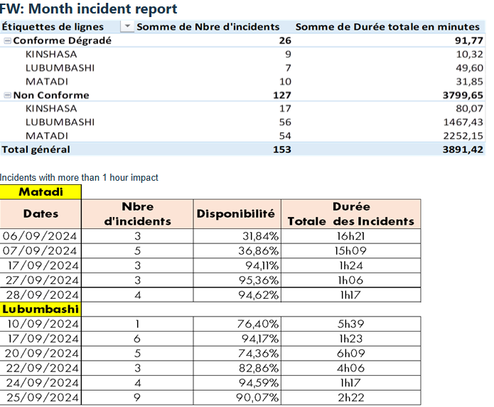
Hi,
What would be the best way to automate this information below? Best would be to get information from Outage list but when exported into excel it’s difficult to use some formulas on the data given.

Best would be to get information from Outage list but when exported into excel it’s difficult to use some formulas on the data given.
DataMiner shows as 20h 15m 15s but I cant set it as a time format to have some formulas working on time to filter out incidents longer than 1 hour and incidents less than an hour.
Can we change the format of this to show hours minutes and seconds as 01:00:00?
On the export DataMiner shows 20h 15m 15s but would be good if the format on the export can be 20:15:15, if it 1d 2h 15m 15s to then be 26:15:15
As this question has now been inactive for a very long time, I will close it. If you still want more information about this, could you post a new question?
Hi Zean
You should be able to extract for example minutes and seconds and convert to proper time using excel formulas.
Did a quick test:
- Assume the data is in cell A1 with the time value 01m 31s
- Use the following formula (ChatGPT did the heavy lifting here…)
=TIMEVALUE(LEFT(A1,FIND(“m”,A1)-1)&”:”&MID(A1,FIND(“m”,A1)+2,FIND(“s”,A1)-FIND(“m”,A1)-2))
- Change the cell format to TIME
Then you should able to perform time calculations.
Hi Wale, this didn't work I got some errors, I tried something else. The issue is if it is one day it displays as 1 day and if it is two or more days it shows as 2 days.
I believe it would be beneficial to have maybe in a hidden column better timing as this causes a lot of opportunity for user error at customers.
I first needed to convert it to seconds and then to time format.
=IFERROR(24*60*60*IF(ISNUMBER(SEARCH(" day";A2));LEFT(A2;SEARCH(" day";A2)-1);IF(ISNUMBER(SEARCH(" days";A2));LEFT(A2;SEARCH(" days";A2)-1);0));0) +
IFERROR(60*60*IF(ISNUMBER(SEARCH("h";A2));MID(A2;IFERROR(SEARCH(" day";A2);IFERROR(SEARCH(" days";A2);0))+5;SEARCH("h";A2)-IFERROR(SEARCH(" day";A2);SEARCH(" days";A2))-5);0);0) +
IFERROR(60*IF(ISNUMBER(SEARCH("m";A2));MID(A2;IFERROR(SEARCH("h";A2);0)+2;SEARCH("m";A2)-IFERROR(SEARCH("h";A2);0)-2);0);0) +
IFERROR(IF(ISNUMBER(SEARCH("s";A2));MID(A2;IFERROR(SEARCH("m";A2);0)+2;SEARCH("s";A2)-IFERROR(SEARCH("m";A2);0)-2);0);0)
then from seconds to correct time format
=TEXT(B2/86400; "[hh]:mm:ss")
Hi, Zean feel free to make a feature suggestion here on Dojo or create a task in collaboration.
Without getting into the weeds of this , for the excel I would approach it slightly differently by first applying a formula to make the format consistent so substitute 'days' for 'day' :
< =SUBSTITUTE(A1, "days", "day") >
then calculate the time value:
< =IFERROR(
VALUE(LEFT(A1,FIND("day",A1&"day")-1))*1 +
VALUE(MID(A1,FIND("day",A1&"day")+3,FIND("h",A1)-FIND("day",A1&"day")-3))/24 +
VALUE(MID(A1,FIND("h",A1)+1,FIND("m",A1)-FIND("h",A1)-1))/1440 +
VALUE(MID(A1,FIND("m",A1)+1,FIND("s",A1)-FIND("m",A1)-1))/86400,
""
) >
then format the cell to display the time as you wish.
Hope it helps.
Hi Zean,
I see that this question has been inactive for some time. Do you still need help with this? If not, could you select the answer (using the ✓ icon) to indicate that no further follow-up is needed?